Loglikelihood of timeseries with Exponential correlation and vector noise.

This example shows how to use tripy.chol_loglike_1D and how it compares to scipy.stats.multivariate_normal for different numbers of observations under the assumption of Exponential correlation.

We assume that the measurements are obtained from the following probabilistic model:

\[\mathbf{X}_{\mathrm{model}}(\mathbf{\theta}) = \mathbf{K}(\boldsymbol{\theta}) \cdot f(\mathbf{t}) + \mathbf{E}_{\mathrm{meas}},\]

where:

• \(\mathbf{X}_{\mathrm{model}}\) is the vector of model predictions.

• \(f(\mathbf{t})\) is a vector valued function.

• \(\mathbf{K}(\boldsymbol{\theta})\) is the correlated multiplicative

uncertainty factor.

• \(\mathbf{E}_{\mathrm{meas}}\) i.i.d. Gaussian random variables.

• \(\boldsymbol{\theta}\) is a set of parameters of the probabilistic model.

The multiplicative factor \(\mathbf{K}\) and additive factor \(\mathbf{E}\)

are distributed as

:math:`mathbf{K}(boldsymbol{theta}) sim mathcal{N} left[ 1.0, boldsymbol{Sigma}_{mathrm{K}}(boldsymbol{theta})

right]`

and :math:`mathbf{E}_{mathrm{meas}} sim mathcal{N}(0,

boldsymbol{Sigma}_{mathrm{E}}`,

respectively. This yields:

\[\mathbf{X}_{\mathrm{model}}(\boldsymbol{\theta}) \sim \mathcal{N} \left[ f(\mathbf{t}), \mathbf{\Sigma}(\boldsymbol{\theta}) \right],\]

with \(\boldsymbol{\Sigma}(\boldsymbol{\theta}) = f(\mathbf{t}) \cdot \boldsymbol{\Sigma}_{\mathrm{K}} + \boldsymbol{\Sigma}_{\mathrm{E}}\)

Import packages:

from timeit import default_timer as timer

import matplotlib.pyplot as plt
import numpy as np
from scipy import stats

from tripy.kernels import Exponential
from tripy.loglikelihood import chol_loglike_1D

Problem setup

N = 100  # Number of points
std_meas = np.repeat(
    2.0, N
)  # Standard deviation of the additive measurement uncertainty
std_model = np.repeat(0.5, N)  # Standard deviation of the modeling uncertainty
l_corr = 10.0  # Correlation lengthscale

# Coordinate vector
t = np.sort(np.linspace(0, 10, N) + 0.1 * np.random.rand(N))

# Vector valued function evaluation
y_func = np.cos(t) + 5

# Observations
v_obs = np.random.rand(N) + y_func

Reference solution using scipy:

e_cov_mx = np.diag(std_meas ** 2)
kernel = Exponential(np.reshape(t, (-1, 1)))
corr_mx = kernel.eval(std_model, length_scale=l_corr)
kph_cov_mx = np.matmul(np.diag(y_func), np.matmul(corr_mx, np.diag(y_func)))
cov_mx = kph_cov_mx + e_cov_mx
logL_ref = stats.multivariate_normal.logpdf(v_obs, cov=cov_mx)

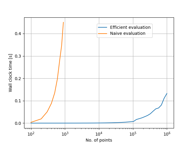
Timing comparison between conventional and efficient solutions:

N_iter = 10

# Reference
N_vec = np.arange(100, 1000, 100)
t_ref_list = []

for i, N in enumerate(N_vec):

    # Vectors of measurement and modeling uncertainty std. dev.
    std_meas = np.repeat(2.0, N)
    std_model = np.repeat(0.5, N)

    # Coord vector and a test function
    t = np.sort(np.linspace(0, 10, N) + 0.1 * np.random.rand(N))
    y_func = np.cos(t) + 5

    # Observations
    v_obs = np.random.rand(N) + y_func

    e_cov_mx = np.diag(std_meas ** 2)
    kernel = Exponential(np.reshape(t, (-1, 1)))

    # Reference
    t1 = timer()
    for _j in range(N_iter):
        corr_mx = kernel.eval(std_model, length_scale=l_corr)
        kph_cov_mx = np.matmul(np.diag(y_func), np.matmul(corr_mx, np.diag(y_func)))
        cov_mx = kph_cov_mx + e_cov_mx
        test = stats.multivariate_normal.logpdf(v_obs, cov=cov_mx)
    t2 = timer()

    t_ref_list.append((t2 - t1) / N_iter)

    print("=============================")
    print(f"Iter {i + 1} / {len(N_vec)}")
    print(f"N = {N}")
    print(f"t = {t_ref_list[-1]}")
    print("=============================")

# Efficient solution
p_vec = np.linspace(2, 6, 50)
t_list = []
for i, p in enumerate(p_vec):

    N = int(10 ** p)

    # Vectors of measurement and modeling uncertainty std. dev.
    std_meas = np.repeat(2.0, N)
    std_model = np.repeat(0.5, N)

    # Coord vector and a test function
    t = np.sort(np.linspace(0, 10, N) + 0.1 * np.random.rand(N))
    y_func = np.cos(t) + 5

    # Observations
    v_obs = np.random.rand(N) + y_func

    # Initial evaluation to perform jit compilation using numba.
    _ = chol_loglike_1D(v_obs, t, l_corr, std_model, std_meas=std_meas, y_model=y_func)

    # Call function
    t1 = timer()
    for _j in range(N_iter):
        test = chol_loglike_1D(
            v_obs, t, l_corr, std_model, std_meas=std_meas, y_model=y_func
        )
    t2 = timer()

    t_list.append((t2 - t1) / N_iter)

    print("=============================")
    print(f"Iter {i + 1} / {len(p_vec)}")
    print(f"p = {p}")
    print(f"t = {t_list[-1]}")
    print("=============================")

=============================
Iter 1 / 9
N = 100
t = 0.0035603168999841727
=============================
=============================
Iter 2 / 9
N = 200
t = 0.018969160400047258
=============================
=============================
Iter 3 / 9
N = 300
t = 0.05043673580003087
=============================
=============================
Iter 4 / 9
N = 400
t = 0.08826102160001029
=============================
=============================
Iter 5 / 9
N = 500
t = 0.13488983229999577
=============================
=============================
Iter 6 / 9
N = 600
t = 0.1975220397999692
=============================
=============================
Iter 7 / 9
N = 700
t = 0.27975037959995463
=============================
=============================
Iter 8 / 9
N = 800
t = 0.3466538785999546
=============================
=============================
Iter 9 / 9
N = 900
t = 0.45019051919998676
=============================
=============================
Iter 1 / 50
p = 2.0
t = 0.00012096610007574781
=============================
=============================
Iter 2 / 50
p = 2.0816326530612246
t = 0.00011933889991269097
=============================
=============================
Iter 3 / 50
p = 2.163265306122449
t = 0.00012152689996582921
=============================
=============================
Iter 4 / 50
p = 2.2448979591836733
t = 0.0001255405999472714
=============================
=============================
Iter 5 / 50
p = 2.326530612244898
t = 0.00012691170004472952
=============================
=============================
Iter 6 / 50
p = 2.4081632653061225
t = 0.00012957170001755004
=============================
=============================
Iter 7 / 50
p = 2.489795918367347
t = 0.0001347796000118251
=============================
=============================
Iter 8 / 50
p = 2.571428571428571
t = 0.00013660829999935232
=============================
=============================
Iter 9 / 50
p = 2.6530612244897958
t = 0.00014357119998749114
=============================
=============================
Iter 10 / 50
p = 2.7346938775510203
t = 0.000153664099980233
=============================
=============================
Iter 11 / 50
p = 2.816326530612245
t = 0.00016326120003213874
=============================
=============================
Iter 12 / 50
p = 2.8979591836734695
t = 0.00016622709999865038
=============================
=============================
Iter 13 / 50
p = 2.979591836734694
t = 0.0001803312999982154
=============================
=============================
Iter 14 / 50
p = 3.061224489795918
t = 0.000191086799986806
=============================
=============================
Iter 15 / 50
p = 3.142857142857143
t = 0.0002030115999332338
=============================
=============================
Iter 16 / 50
p = 3.224489795918367
t = 0.00022316880003927508
=============================
=============================
Iter 17 / 50
p = 3.3061224489795915
t = 0.0002450143000714888
=============================
=============================
Iter 18 / 50
p = 3.387755102040816
t = 0.00026978089999829535
=============================
=============================
Iter 19 / 50
p = 3.4693877551020407
t = 0.000300571800016769
=============================
=============================
Iter 20 / 50
p = 3.5510204081632653
t = 0.00039793039995856817
=============================
=============================
Iter 21 / 50
p = 3.63265306122449
t = 0.0003884934999405232
=============================
=============================
Iter 22 / 50
p = 3.7142857142857144
t = 0.00045730729998467724
=============================
=============================
Iter 23 / 50
p = 3.7959183673469385
t = 0.0005125417999806813
=============================
=============================
Iter 24 / 50
p = 3.877551020408163
t = 0.000601132400061033
=============================
=============================
Iter 25 / 50
p = 3.9591836734693877
t = 0.0007057223000629165
=============================
=============================
Iter 26 / 50
p = 4.040816326530612
t = 0.0008264666000286525
=============================
=============================
Iter 27 / 50
p = 4.122448979591836
t = 0.0009909420999974828
=============================
=============================
Iter 28 / 50
p = 4.204081632653061
t = 0.0011400579999644833
=============================
=============================
Iter 29 / 50
p = 4.285714285714286
t = 0.0014041727000403625
=============================
=============================
Iter 30 / 50
p = 4.36734693877551
t = 0.0016396580999753496
=============================
=============================
Iter 31 / 50
p = 4.448979591836734
t = 0.0019787538999480603
=============================
=============================
Iter 32 / 50
p = 4.530612244897959
t = 0.0023910080000860033
=============================
=============================
Iter 33 / 50
p = 4.612244897959183
t = 0.002953916099977505
=============================
=============================
Iter 34 / 50
p = 4.6938775510204085
t = 0.003536905800046952
=============================
=============================
Iter 35 / 50
p = 4.775510204081632
t = 0.004306851899946196
=============================
=============================
Iter 36 / 50
p = 4.857142857142857
t = 0.005320713099990826
=============================
=============================
Iter 37 / 50
p = 4.938775510204081
t = 0.006347501300024305
=============================
=============================
Iter 38 / 50
p = 5.020408163265306
t = 0.007759314099985204
=============================
=============================
Iter 39 / 50
p = 5.1020408163265305
t = 0.016246511600002123
=============================
=============================
Iter 40 / 50
p = 5.183673469387754
t = 0.019905919499979063
=============================
=============================
Iter 41 / 50
p = 5.26530612244898
t = 0.02375712110006134
=============================
=============================
Iter 42 / 50
p = 5.346938775510203
t = 0.028778146900003777
=============================
=============================
Iter 43 / 50
p = 5.428571428571429
t = 0.03418520909999643
=============================
=============================
Iter 44 / 50
p = 5.5102040816326525
t = 0.04164081749995603
=============================
=============================
Iter 45 / 50
p = 5.591836734693877
t = 0.053113126900007045
=============================
=============================
Iter 46 / 50
p = 5.673469387755102
t = 0.06383499880003
=============================
=============================
Iter 47 / 50
p = 5.755102040816326
t = 0.06773462769997422
=============================
=============================
Iter 48 / 50
p = 5.836734693877551
t = 0.08074620279994633
=============================
=============================
Iter 49 / 50
p = 5.918367346938775
t = 0.11114553600000363
=============================
=============================
Iter 50 / 50
p = 6.0
t = 0.13258634270005132
=============================

Plot a comparison of the wall clock times:

fig = plt.figure()
plt.plot([int(10 ** p) for p in p_vec], t_list, label="Efficient evaluation")
plt.plot(N_vec, t_ref_list, label="Naive evaluation")
plt.xlabel("No. of points")
plt.ylabel("Wall clock time [s]")
plt.xscale("log")
plt.legend(bbox_to_anchor=(0.8, 0.85), bbox_transform=fig.transFigure)
plt.grid()
plt.show()